Commercial solar ROI should be calculated from the project’s long-term cash flow, not from a simple comparison between the system price and the customer’s current annual electricity bill. When I assess a factory, warehouse, hotel, farm, or commercial building, I separate the electricity generated by the system from the financial value that the customer can actually capture. Some solar electricity replaces expensive grid purchases, some may be exported at a lower rate, and some may be curtailed because the site cannot consume or export it. I then account for operating expenses, degradation, financing, taxes, incentives, equipment replacement, and the time value of money. Only after these variables are defined can I present a payback period, net present value, internal rate of return, or lifetime savings figure that has real commercial meaning.
The industry problem is that many sales proposals show one attractive payback number without revealing the assumptions behind it. A five-year payback can appear convincing, but it may depend on unrealistic annual generation, one hundred percent self-consumption, rapidly increasing electricity prices, no maintenance expenses, no equipment replacement, and full eligibility for incentives that have not been confirmed. I prefer to show how the result was constructed and how it changes under different operating and financial scenarios. In my experience, a transparent seven-year estimate is more useful than an unsupported four-year promise because the customer can understand the risks and make a defensible investment decision.
Why the Electricity Bill Alone Cannot Determine ROI
The electricity bill provides an essential starting point, but I never assume that the solar system can eliminate the entire amount. A commercial bill may contain energy charges, demand charges, fixed connection fees, reactive-power penalties, taxes, capacity charges, and other tariff components. Solar generation may reduce some of these charges substantially while leaving others almost unchanged. If I calculate savings by multiplying annual solar production by the average amount shown on the bill, I may assign the same value to every kilowatt-hour even though the tariff treats consumption differently by time, demand level, or billing category.
I therefore reconstruct the bill before estimating savings. I identify the energy rate applied during solar-production hours, the value of exported electricity, the demand-charge methodology, and any fixed charges that continue after the system is installed. I also review whether installing solar could move the customer to another tariff or change the way import and export are settled. Utility rate design can materially alter commercial PV economics, and the absence or structure of net metering can affect the economically attractive project size.
Annual Solar Production Is the First Input, Not the Final Saving
I begin the energy side of the analysis with the expected annual AC electricity delivered by the system. This should come from a site-specific production model that reflects the project location, module orientation, tilt, temperature, shading, soiling, inverter efficiency, cable losses, transformer losses where applicable, equipment availability, and the proposed DC-to-AC ratio. I do not calculate ROI from the total module nameplate rating alone because a 500 kWp array does not produce 500 kW continuously, nor does it generate the same annual energy in every location.
The first-year production estimate should also be presented as an engineering forecast rather than a guarantee. Weather varies from year to year, site conditions may differ from preliminary assumptions, and actual operating availability depends on maintenance and fault response. I therefore prefer to show the modeled annual production, the principal loss assumptions, and a sensitivity range. This makes it possible to distinguish between the project’s expected outcome and a more conservative case if generation is lower than forecast.
Self-Consumption Determines the Value of Each Generated Kilowatt-Hour
The self-consumption percentage tells me how much of the solar electricity is used directly by the facility rather than exported or curtailed. I consider this one of the most influential variables in commercial solar ROI because electricity consumed onsite normally replaces grid electricity at the applicable import tariff, while exported electricity may receive a lower price or no compensation.
Suppose a system generates 800,000 kWh in its first year. If the factory consumes 90 percent onsite and exports 10 percent, then 720,000 kWh creates value by reducing grid purchases, while 80,000 kWh is valued according to the export arrangement. If another factory uses only 55 percent onsite, the same system and annual production can produce a very different financial result. The difference does not come from the panels or inverter; it comes from how the facility’s load overlaps with solar production.
I calculate self-consumption by comparing interval load data with simulated solar output, ideally in 15-minute, 30-minute, or hourly periods. Monthly electricity totals are not sufficient because they can hide low daytime demand, weekends, holidays, production shutdowns, and seasonal changes. A site can consume more energy annually than the PV system produces and still export substantial midday power if much of its electricity use occurs at night.
Self-Consumption and Solar Coverage Must Not Be Confused
I separate the self-consumption ratio from the solar-coverage ratio because they answer different questions. The self-consumption ratio shows what percentage of generated solar electricity is used onsite. The solar-coverage ratio shows what percentage of the facility’s total electricity demand is supplied by solar.
A relatively small system may achieve nearly complete self-consumption because the site always has enough daytime load to absorb its output, yet it may cover only a modest share of annual demand. A larger system may cover more of the customer’s electricity use but export or curtail a greater percentage of generation. Neither result is automatically better. The preferred balance depends on the value of imported electricity, export compensation, available space, capital budget, and the customer’s objective.
I show both measurements because a proposal stating “90 percent solar utilization” can be misleading when it does not explain whether that means 90 percent of solar generation is consumed onsite or solar covers 90 percent of the building’s electricity. Those are entirely different commercial outcomes.
How I Calculate the First-Year Electricity Saving
I calculate the basic first-year energy saving by separating onsite solar consumption from exported generation. The value of onsite consumption is determined by the grid electricity charges that are genuinely avoided during the periods when solar is operating. The value of exported electricity is determined by the applicable feed-in tariff, net-metering credit, wholesale rate, or contractual export price.
For example, suppose a system generates 1,000,000 kWh in the first year. If 800,000 kWh is consumed onsite and replaces electricity costing $0.15 per kWh, the avoided energy-purchase value is approximately $120,000. If the remaining 200,000 kWh is exported at $0.05 per kWh, it adds approximately $10,000. The gross first-year energy value would therefore be approximately $130,000 before considering demand-charge effects, operating costs, financing, taxes, curtailment, and degradation.
I use this type of separated calculation rather than multiplying the complete 1,000,000 kWh by $0.15, which would incorrectly value exported electricity as though it offset the retail tariff. In this example, that shortcut would overstate annual value by about $20,000 before any other assumptions were considered.
Electricity Tariffs Must Be Modeled by Time and Charge Type
Commercial tariffs can include different energy prices at peak, shoulder, and off-peak periods. I therefore assign solar savings according to the tariff that applies when the electricity is generated and consumed. A kilowatt-hour produced during an expensive afternoon peak period may be worth more than one produced during a low-rate period. If the utility uses seasonal tariffs, the same solar output can also have different values in summer and winter.
I also examine how tariffs may change over time, but I avoid assuming aggressive electricity-price inflation merely to improve the ROI. I normally show a base escalation assumption and test lower and higher scenarios. A project that works only when electricity prices rise rapidly carries more financial risk than one that remains attractive under stable or moderately increasing rates.
When future tariff policy is uncertain, I make that uncertainty visible. Net-metering rules, export rates, and demand-charge structures can change over the operating life of a project. I therefore distinguish contractual or approved tariff conditions from assumptions about future regulatory treatment.
Demand Charges Require a Separate Calculation
Demand charges are commonly based on the customer’s highest measured power demand during a billing interval rather than the total energy consumed. I do not assume that solar generation will reduce demand charges in the same proportion as energy charges because the facility’s billing peak may occur when solar output is low or unavailable.
If the customer’s maximum demand occurs on a sunny afternoon and remains relatively consistent, solar may reduce the recorded peak. If the peak occurs after sunset, during a cloudy production surge, or when a large motor starts, a standard PV system may have little effect. The result depends on the utility’s demand-measurement interval, ratchet clauses, seasonal rules, coincident or non-coincident demand structure, and the facility’s operating pattern.
I therefore model demand savings using interval load and solar-production data whenever demand charges represent a meaningful part of the bill. I avoid promising that a 500 kW inverter will reduce billed demand by 500 kW because inverter capacity and demand-charge reduction are not equivalent. Solar output varies, and the billing peak may not coincide with the plant’s maximum generation.
Export Compensation Can Change the Optimal System Size
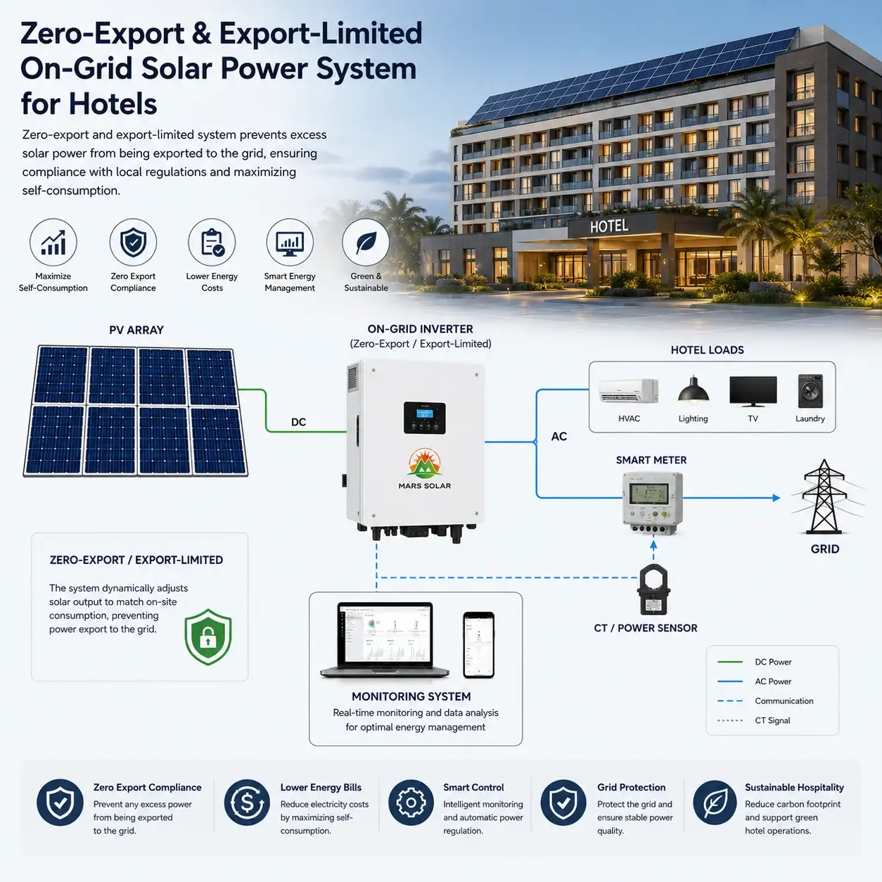
Exported electricity should be valued according to the actual approved compensation mechanism. Under some arrangements, eligible exports may receive a credit close to the retail energy rate. Under others, the payment may be substantially lower. Some sites may receive no payment or may be prohibited from exporting altogether.
This difference influences both ROI and system sizing. When export compensation is attractive, installing more capacity than the site can consume at certain times may still produce commercial value. When exported electricity has little value, I normally place greater emphasis on daytime self-consumption. A system designed to fill the entire roof may generate more annual energy but deliver a weaker return on the final portion of installed capacity.
I test the marginal value of added capacity rather than assuming that every additional module produces the same financial benefit. The first part of the array may offset high-value onsite consumption, while later additions increasingly produce low-value export. This is why the largest technically possible system is not always the financially optimal one.
Curtailment Must Be Deducted from Usable Generation
Curtailment occurs when the system is capable of generating electricity but is instructed or forced to reduce output. In a zero-export installation, the controller may curtail generation when PV output exceeds onsite demand. In an export-limited project, output may be reduced whenever the approved export ceiling is reached. A utility or plant controller may also impose temporary limits for grid-management reasons.
I calculate ROI from the electricity that can actually be used or sold, not from unconstrained theoretical production. If a system could generate 1,000,000 kWh but is expected to curtail 80,000 kWh, only the remaining 920,000 kWh should enter the initial savings calculation. I then divide that output between self-consumed and exported energy.
Curtailment is particularly important for factories that close on weekends or experience seasonal production shutdowns. A high monthly electricity bill can create the impression that a large system will be fully utilized, while interval modeling reveals long periods when the site load is too low. Ignoring these periods can make the projected ROI appear much stronger than the actual operating result.
Inverter Clipping and Export Curtailment Are Different Losses
I separate inverter clipping from control-based curtailment because they arise from different design decisions. Clipping occurs when the DC array could provide more power than the inverter can convert at its rated AC output. Curtailment occurs when the inverter could produce more AC power but is intentionally limited by the export controller, utility, or site operating strategy.
A moderate amount of clipping can be economically justified when additional module capacity improves output during mornings, afternoons, cloudy periods, and lower-irradiance seasons. Curtailment caused by low site demand may provide less value because the additional generation cannot be consumed or exported. A project can experience both losses, so combining them into one general percentage makes it difficult to understand whether changing the module quantity, inverter capacity, export limit, or operating schedule would improve the result.
I therefore show each loss separately in the energy model and explain what controls it. This helps the buyer see whether lost production is an intentional economic trade-off or a consequence of grid and load constraints.
Module Degradation Changes Savings Over Time
Solar modules gradually lose output over their operating life, so I do not repeat the first-year generation figure unchanged across a 20- or 25-year financial model. I apply a degradation assumption based on the module technology, manufacturer information, performance warranty, site conditions, and credible engineering data.
If first-year generation is 1,000,000 kWh and the model uses annual degradation, each later year begins with slightly less expected production. The financial effect depends on tariff escalation and operating conditions. Electricity prices may increase while energy production declines, meaning annual savings can still rise in nominal terms even though the system generates less electricity.
I show degradation explicitly because omitting it overstates lifetime generation and savings. I also avoid claiming that the performance-warranty endpoint predicts the exact annual degradation path. A warranty provides a contractual threshold under specified terms; it is not a guarantee that every system will follow one perfectly smooth performance curve.
O&M Expenses Must Be Included Even When Solar Is Low-Maintenance
Commercial PV systems generally require less routine maintenance than many conventional energy assets, but they are not cost-free. I include expected expenses for inspections, cleaning where necessary, monitoring, vegetation control for ground-mounted systems, testing, communications, insurance, security, corrective maintenance, and specialist labour.
The appropriate O&M allowance depends on project scale, environment, equipment architecture, access, service agreement, and local labour cost. A dusty industrial site may require more frequent cleaning than a well-rained rooftop. A remote solar farm may face higher travel and spare-parts costs than an urban commercial building. A multi-inverter system may provide easier fault isolation but involve more individual devices, fans, communication modules, and protective components.
NREL describes O&M as recurring expenditure required to operate and maintain a PV plant over its lifetime, reinforcing why these costs belong in the cash-flow model rather than being treated as an unexpected future deduction.
Equipment Replacement Assumptions Must Be Realistic
A commercial financial model should consider whether major components may require replacement or substantial repair during the project life. I do not assume that every inverter will fail in one predetermined year, but I normally include an allowance based on product warranty, design life, serviceability, environmental conditions, redundancy, and replacement cost.
Inverter replacement is particularly important because module warranties may extend much longer than the standard product warranty of some power-electronic equipment. Communication devices, data loggers, surge-protection cartridges, fans, meters, and other auxiliary components may also require replacement. Transformer and switchgear maintenance may become relevant for larger plants.
Historical NREL feasibility models have included both annual O&M and future inverter replacement assumptions, illustrating why a lifecycle analysis should extend beyond the initial purchase. I use project-specific assumptions rather than copying old benchmark costs, but the financial principle remains valid: equipment that may need replacement should be represented in future cash flow.
Financing Changes Both Cash Flow and ROI
The way the project is financed can change the customer’s cash flow even when the technical system is identical. A cash purchase requires a large initial expenditure but avoids loan interest. A bank loan spreads the cost over time but introduces interest, fees, repayment schedules, security requirements, and possibly a required debt-service reserve. A lease or power purchase agreement may reduce initial capital requirements but changes ownership, tax benefits, contract obligations, and the way savings are measured.
I distinguish project ROI from equity ROI. Project ROI evaluates the economic performance of the asset before considering the financing structure, while equity returns evaluate the cash invested by the owner after debt and financing costs. Leverage can improve the equity IRR when the project return exceeds the cost of borrowing, but it can also increase risk when actual savings fall below projections.
Payback also changes under financing. The customer may achieve positive cash flow from the first year if annual utility savings exceed annual payments, even though the system has not “paid for itself” in the same sense as a cash purchase. DOE similarly distinguishes cash purchase, loan, and PPA structures when explaining solar savings and payback.
Tax Treatment Must Be Modeled for the Customer’s Jurisdiction
Taxes can materially affect commercial solar returns, but I never apply a generic tax benefit across every country or customer. The analysis may need to consider depreciation, investment credits, accelerated allowances, deductible interest, value-added tax, import duties, corporate income tax, withholding tax, property tax, and the tax treatment of export revenue.
The correct treatment depends on project ownership, location, entity structure, placed-in-service date, financing arrangement, and current legislation. In the United States, for example, clean-electricity investment incentives have specific qualification rules, tax forms, bonus provisions, and compliance requirements that need to be checked against current IRS guidance rather than assumed from an older sales proposal.
I normally calculate a pre-tax project case first and then add an after-tax case prepared or verified with the customer’s accountant or tax adviser. This prevents an uncertain incentive from being hidden inside the core technical economics.
Incentives Should Be Confirmed Rather Than Assumed
Grants, rebates, tax credits, renewable-energy certificates, low-interest loans, accelerated depreciation, and other incentives can shorten payback considerably. I include them only when the project appears eligible and the customer understands the application conditions, timing, caps, documentation, and risk of non-approval.
A sales quotation may state an attractive net price after incentives as though the benefit were automatic. In reality, the customer may need to apply before ordering, use approved equipment, meet labour or content requirements, complete the project by a deadline, or wait for reimbursement after commissioning. The incentive may also reduce the tax basis used for depreciation or interact with other programs.
I therefore show the gross project cost, confirmed incentive, expected net investment, and any unconfirmed incentive scenario separately. The project should ideally remain understandable without relying on an uncertain benefit.
Inflation and Electricity-Price Escalation Must Be Applied Consistently
Long-term models frequently use nominal cash flows, which include expected inflation, or real cash flows, which remove general inflation. I choose one framework and use it consistently. If electricity tariffs, O&M costs, replacement expenses, and discount rates are mixed between nominal and real assumptions, the resulting NPV and IRR can become misleading.
I normally state the assumed annual electricity-price escalation, O&M escalation, general inflation, and discount rate clearly. I also test a scenario with lower tariff growth because electricity-price forecasts are uncertain and regulatory changes can affect future rates.
An attractive project should not depend entirely on one aggressive escalation figure. If a small change in tariff growth turns the NPV from strongly positive to negative, the buyer should understand that sensitivity before investing.
Simple Payback Is Useful but Incomplete
Simple payback measures how long cumulative net savings take to recover the initial investment. If a project costs $700,000 and produces $100,000 of net savings each year, a simple calculation suggests a seven-year payback. I use this metric because it is easy for decision-makers to understand, but I do not rely on it alone.
Simple payback often ignores the timing of cash flows, financing, degradation, replacement costs, taxes, incentives, and the value created after the payback year. Two projects can have the same payback but very different lifetime profitability. One may continue generating strong savings for twenty years, while another may face major replacement expenses soon after payback.
I therefore present payback as one indicator rather than the complete investment conclusion. DOE defines payback for a cash-purchased solar system as the period required for the system to recover its cost, but broader commercial analysis still requires other financial measures.
Net Present Value Shows the Value Created in Today’s Money
Net present value allows me to compare future cash flows with the initial investment by discounting future savings and costs to their present value. I calculate the annual net cash flow from electricity savings, export revenue, incentives, tax effects, O&M, financing where relevant, and equipment replacement, then discount each year using an appropriate rate.
A positive NPV indicates that the modeled project creates value above the required return represented by the discount rate. A negative NPV indicates that the projected benefits do not recover the investment and required return under those assumptions.
I consider NPV more informative than simple payback because it recognizes that money received in year fifteen is worth less than money received today and includes the project’s full operating life. However, the result is sensitive to the chosen discount rate, so I show that assumption clearly rather than presenting NPV as an objective value independent of the investor’s cost of capital and risk expectations.
Internal Rate of Return Helps Compare Investment Opportunities
The internal rate of return is the discount rate at which the project’s NPV equals zero. I use IRR to help customers compare solar with other investment opportunities, although it should be reviewed together with NPV, project scale, financing structure, and risk.
A smaller project can have a high IRR but create less total financial value than a larger project with a slightly lower IRR. Projects with unusual cash-flow patterns can also produce less intuitive IRR results. For this reason, I do not rank every proposal by IRR alone.
NREL’s System Advisor Model guidance describes IRR through the point where NPV changes from positive to negative, which reflects the direct relationship between these two financial measures. I use the metric within a complete cash-flow model rather than calculating it from only the system price and first-year saving.
Lifetime Savings Must Be Presented as Net Cash Flow
Lifetime savings should represent the cumulative financial benefit after relevant expenses rather than simply multiplying first-year electricity savings by the number of operating years. I include the annual change in production, tariff assumptions, export value, O&M costs, replacement expenses, financing payments, taxes, incentives, and any terminal or decommissioning assumptions.
For example, a project may create $150,000 of gross energy value in year one but require $12,000 of O&M and insurance. A future inverter replacement may create a major negative cash flow in a later year. Tariff escalation may increase nominal savings, while degradation reduces physical generation. The cumulative net benefit should reflect all of these movements.
I normally present a year-by-year cash-flow table and a cumulative cash-flow curve. This allows the buyer to see when the project becomes cash-positive, whether replacement costs create temporary reversals, and how much value is expected after simple payback.
A Practical Commercial Solar ROI Example
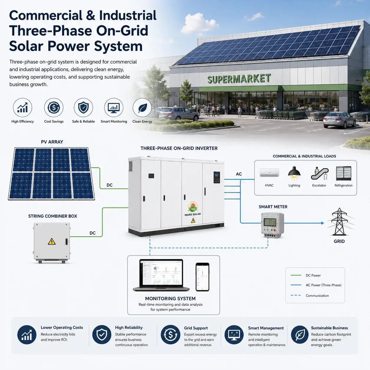
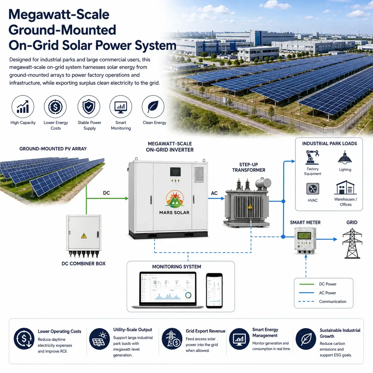
Consider a factory evaluating a 500 kW AC on-grid system with a larger DC module array. Assume the modeled first-year generation is 850,000 kWh after system losses. Based on interval data, 80 percent of that generation, or 680,000 kWh, is expected to be consumed onsite, while 15 percent, or 127,500 kWh, is exported. The remaining 5 percent, or 42,500 kWh, is expected to be curtailed because of low-load periods and the project’s export limit.
If onsite consumption avoids an average energy charge of $0.14 per kWh, its first-year energy value is approximately $95,200. If exported electricity is compensated at $0.05 per kWh, it adds approximately $6,375. If modeled demand-charge reduction adds another $8,000, total gross first-year benefit becomes approximately $109,575.
If annual O&M, monitoring, insurance, and administration total $12,000, the first-year operating benefit before financing and tax is approximately $97,575. If the installed project cost is $650,000 after confirmed incentives, a rough simple-payback estimate would be about 6.7 years. However, I would not stop there. I would model annual degradation, tariff escalation, O&M escalation, possible inverter replacement, financing, taxes, and the investor’s discount rate to calculate NPV, IRR, and cumulative cash flow.
This example is illustrative rather than a universal benchmark. Its purpose is to show how annual generation becomes financial value only after self-consumption, export, curtailment, tariff, demand, and operating costs are separated.
How One Assumption Can Change the Entire Result
Using the same example, suppose the self-consumption estimate falls from 80 percent to 60 percent because the factory operates fewer daytime shifts than initially reported. An additional 170,000 kWh would move from high-value onsite use to export or curtailment. If that energy is exported at $0.05 instead of offsetting grid purchases at $0.14, the value falls by $0.09 per kWh, reducing annual benefit by approximately $15,300 before considering any increase in curtailment.
If electricity-price escalation is also lower than expected, the lifetime NPV falls further. If the project qualifies for a larger confirmed incentive or the customer adds a daytime production line, the result may improve. This is why one payback number without assumptions has limited value.
I normally test at least a base case, conservative case, and stronger-performance case. The conservative scenario may use lower generation, lower self-consumption, lower tariff escalation, higher O&M, and a higher discount rate. The purpose is not to make the project look weak; it is to show whether the investment remains acceptable when reality differs from the central forecast.
How I Build a Credible Sensitivity Analysis
A useful sensitivity analysis changes the assumptions that genuinely drive project value. I focus on annual production, self-consumption, import tariff, export compensation, curtailment, installed cost, O&M, financing rate, degradation, replacement expense, and discount rate.
I avoid changing every variable simultaneously without explanation because the buyer then cannot see which risk matters most. Instead, I show how the result responds to one or two important variables and identify the break-even point. For example, I may calculate the minimum self-consumption rate required to achieve the target IRR or the maximum installed cost that keeps payback below the customer’s investment limit.
This process can also influence design. If ROI is highly sensitive to export compensation, a smaller array may be safer. If the project remains strong even with lower generation, the investment may be more resilient. If demand-charge savings drive most of the value, interval analysis and tariff verification deserve additional attention before approval.
Why Optimistic Sales Payback Figures Often Fail
The most common optimistic models assume that every generated kilowatt-hour offsets the full retail tariff, the system operates without curtailment, electricity prices rise rapidly, modules do not degrade, and maintenance or replacement costs are negligible. Some models also subtract an incentive before confirming eligibility or compare the project price with the entire electricity bill, including fixed charges that solar cannot eliminate.
These assumptions can make a quotation look commercially impressive while shifting the risk to the buyer. The problem may not appear in the first months because generation is visible and the bill decreases, but the actual annual saving can still fall below the promised figure.
I consider a financial proposal credible when the assumptions are traceable to electricity bills, interval data, production modeling, utility tariffs, export rules, equipment warranties, financing terms, and confirmed incentives. When one figure cannot be explained, I do not allow it to carry the investment decision.
What a Professional ROI Report Should Explain
A professional commercial solar financial analysis should allow the reader to follow the complete path from energy production to investment return. I explain the DC and AC capacities, first-year generation, annual degradation, self-consumption, export, curtailment, import and export tariffs, demand-charge effects, O&M, replacement assumptions, project cost, incentives, financing, tax treatment, discount rate, payback, NPV, IRR, and lifetime net benefit.
I also state which inputs are confirmed, which come from engineering models, and which remain financial assumptions. This distinction matters because a utility tariff shown on a current bill is more certain than a forecast of electricity prices fifteen years into the future.
The report should make it possible for another engineer, financial manager, lender, or investor to review the logic without relying on the salesperson’s verbal explanation. In my view, transparency is not an extra feature of the financial model; it is what makes the result commercially usable.
Commercial Solar ROI Is a Range, Not a Promise
I treat solar ROI as a modeled range based on defined assumptions rather than a guaranteed number. The system’s performance depends on weather, equipment availability, site operations, tariff changes, export rules, maintenance, and the customer’s actual load. A reliable analysis reduces uncertainty, but it cannot remove every future variable.
The strongest projects are usually those that remain financially attractive under conservative assumptions. They do not depend entirely on maximum production, perfect self-consumption, high export rates, or uncertain incentives. Their value comes from a clear match between daytime demand, solar output, electricity cost, system design, and long-term operating discipline.
When I calculate commercial solar savings, my objective is not to produce the shortest possible payback period. My objective is to show how the investment is expected to perform, which assumptions matter most, where the risks are located, and what must happen for the customer to achieve the projected return.